Color Invariance using Linear Image Filters

The problem with recognizing general shapes, such as balls, as in our particular case, is the number of possibilities in the visual appearance of a ball. A ball can take on any color, size and may have any pattern on its surface. In order to generalize the concept of a ball, the initial goal was the elimination of any color information in the data images representing the balls.

In this paper, we have achieved this using linear image filters to detect the edges in the image, followed by a threshold to eliminate noise data, which would then be given as input to the classifier, which in turn handles differences in size, pattern, lighting, etc.

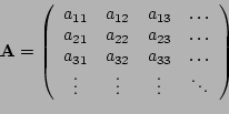
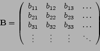
The most common edge detection techniques used are gradient and Laplacian operators. For this paper, we have experimented with multiple gradient filters, as well as a Laplacian filter, which we implemented ourselves, according to the algorithm described in [3]. The technique of the gradient operator is defined as follows:

$$\mathbf{A} = \left( \begin{array}{cccc} a_{11} & a_{12} & a_... ...ldots \\ \vdots & \vdots & \vdots & \ddots \end{array}\right)$$

$$\mathbf{B} = \left( \begin{array}{cccc} b_{11} & b_{12} & b_... ...ldots \\ \vdots & \vdots & \vdots & \ddots \end{array}\right)$$

$$\mathbf{V} = \left( \begin{array}{ccc} v_{11} & v_{12} & v_{13} \\ v_{21} & v_{22} & v_{23} \\ v_{31} & v_{32} & v_{33} \end{array} \right) \mathbf{H} = \left( \begin{array}{ccc} h_{11} & h_{12} & h_{13} \\ h_{21} & h_{22} & h_{23} \\ h_{31} & h_{32} & h_{33} \end{array} \right)$$

$$v_{i,j} = \sum_{x=i-1}^{i+1} \sum_{y=j-1}^{j+1} v$$ (1)

$$end{tex2html_deferred}_factor * a_{x, y} * v_{x, y}$$

$$end{tex2html_deferred}$$ (2)

$$end{tex2html_deferred} h_{i,j} = \sum_{x=i-1}^{i+1} \sum_{y=j-1}^{j+1} h$$ (3)

$$end{tex2html_deferred}_factor * a_{x, y} * h_{x, y}$$ (4)

$$end{tex2html_deferred}$$ (5)

$$end{tex2html_deferred} b_{i,j} = \sqrt{(v_{i,j}^2 + h_{i,j}^2) * edge$$ (6)

$$end{tex2html_deferred}_intensity{$$

where $A$ represents the matrix of pixels in the input image, $B$ the output image and $V$ and $H$ the $3\times 3$ vertical and horizontal masks that are moved over the image pixels starting at the top left corner, through to the bottom right. A number of parameters need to be adjusted for each filter instance, such as the $edge\_intensity$, which defines how ``thick'' the output edges should be, and $h\_factor$ and $v\_factor$ to emphasize the differentiation in each direction (horizontal or vertical, respectively).

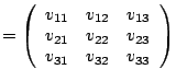
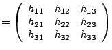
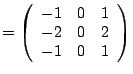
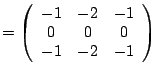
In our approach, we used a Sobel filter, with $V$ and $H$ defined below, $edge\_intensity = 4.0$ and both $v\_factor$ and $h\_factor$ equal to $1$.

$$\mathbf{V} = \left( \begin{array}{ccc} -1 & 0 & 1 \\ -2 & 0 & 2 \\ -1 & 0 & 1 \end{array} \right) \mathbf{H} = \left( \begin{array}{ccc} -1 & -2 & -1 \\ 0 & 0 & 0 \\ -1 & -2 & -1 \end{array} \right)$$

Two techniques were attempted in terms of filtering and thresholding:

• Converting the image into gray scale mode and then applying the filtering algorithm, followed by the threshold.
• Applying the filter to the colored image and then using a threshold to include any pixel in any of the 3 color channels that crossed the threshold value in the output image.

The difference in results is shown in Fig. 2. A typical output of the Sobel filter is shown in Fig. 3.

Figure 2: Left: A Sobel filter applied to a gray scale image. Right: Sobel filter applied to a colored image and then thresholded.

Figure 3: Typical output of the Sobel filter

This edge detection and thresholding technique is applied to all images used as input to the training of the Haar classifier. The training process itself is illustrated in the following subsections.