Matching Sewerage Pipes

Inspecting communal sewer systems is a potential application for mobile robots  [3,14]. Two basic problems of such inspection robots are self localization and the reconstruction of sewerage pipe system. These two problems are addressed in this section. Similar to matching sewerage pipes is the problem of mapping cylinders in 3D data, which is well known in the reconstruction of industrial environments with pipes and tubes [5]. State of the art is semi-automatic reconstruction [9].

Figure: A sewerage pipe is modeled by two points $\V a$ and $\V b$ and the radius $r$.

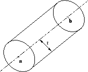
For matching of tubes into scanned pipes, the closest point on the pipe surface is calculated as follows: Given a scan point $\V x \in \R ^3$ and a pipe, described by two points $\V a$ and $\V b$ ( $\V a, \V b \in \R ^3$) and the radius $r$ (figure 7), the closest point $\V c$ to $\V x$ on the pipe surface is

$$\V n = \frac{\V a - \V b}{$$ (2)

$$end{tex2html_deferred}\vert \V a - \V b$$ (3)

$$end{tex2html_deferred}\vert{$$ (4)

$$end{tex2html_deferred} \qquad s = \frac{<\V x, \V n>}{<\V n, \V n>}$$ (5)

$$end{tex2html_deferred}$$ (6)

$$end{tex2html_deferred} \V c = s\cdot\V n + r\cdot \frac{\V x - s \cdot \V n}{\left$$ (7)

$$end{tex2html_deferred}\vert\V x - s \cdot \V n\right$$ (8)

$$end{tex2html_deferred}\vert{$$ (9)

with $\V n$ the norm vector between $\V a$ and $\V b$ and $s$ the projection of $\V x$ to $\V n$.

The following steps match pipes with the pipe model:

1. A default tube is inserted into the 3D scan to initialize the matching (figure 8 top left).
2. An optimal rotation and translation matrix is calculated with the ICP algorithm (figure 8 top right).
3. The radius of the tube is gradually enlarged or reduced until the tube matches the 3D points, i.e., until the error function of the ICP algorithm is minimal (figure 8 bottom).

At the beginning, the last two steps are iterated with a reduced number of points to rapidly calculate the transformations. Finally the matching is refined with all points. The result is given in figure 8 and 9.

Figure 8: Matching of a tube into a scanned sewerage pipe (first the tube is being rotated & translated into the correct position, then the size is being adapted)

Figure 9: Distances between scanned points and ideal tube. Left: A tube with point-to-tube vectors and without adjusted radius. Middle: Fully processed tube with an obstacle (a brick). Right: KURT2 inside of a test sewer network.

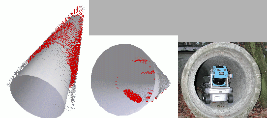
With the proposed matching, a pipe is reconstructed. Due to the exact matching of the tube and the high precision of the scanner, deviations and abnormalities like pipe deformations are also detected. Furthermore obstacles, e.g., a brick as given in the middle picture of figure 9 are found. The self localization of the robot is improved, because the transformations calculated by the matching process is applied to the robot pose.