Extracting Semantic Information

The basic idea of labelling 3D points with semantic information is to use the gradient between neighbouring points to differ between three categories, i.e., floor-, object- and ceiling-points. A 3D point cloud that is scanned in a yawing scan configuration, can be described as a set of points $\V p_{i,j} = (\phi_i,r_{i,j},z_{i,j})^T$ given in a cylindrical coordinate system, with $i$ the index of a vertical raw scan and $j$ the point index within one vertical raw scan counting bottom up. The gradient $\alpha_{i,j}$ is calculated by the following equation:

$$\tan \alpha_{i,j}= \frac{z_{i,j}-z_{i,j-1}}{r_{i,j}-r_{i,j-1}} \quad -\frac{1}{2}\pi \leq \alpha_{i,j} < \frac{3}{2}\pi.$$

The classification of point $\V p_{i,j}$ is directly derived from the gradient $\alpha_{i,j}$:

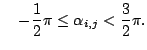
 1. ceiling-points: ¯
 1.   floor-points:  
$\alpha_{i,j} < \tau$


2.   object-points: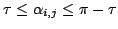  
$\tau \leq \alpha_{i,j} \leq \pi - \tau$ 


3.   ceiling-points:  
$\pi - \tau < \alpha_{i,j}$

with a constant $\tau$ that depends on the maximal ascent being accessible by the robot (here: $\tau = 20^\circ$).

Applied to real data, this simple definition causes two problems. As can be seen in Fig. (a) noisy range data can lead to wrong classifications of floor- and ceiling-points. Changing the differential quotient as follows solves this problem:

$$\tan \alpha_{i,j}= \frac{z_{i,j}-z_{i,j-k}}{r_{i,j}-r_{i,j-k}}$$

with $k \in \N , k \geq 1$ the smallest number so that

$$\sqrt{(r_{i,j} - r_{i,j-k})^2+(z_{i,j} - z_{i,j-k})^2} > d_{\text{min}}$$

for a constant $d_{\text{min}}$ depending on the scanner's depth accuracy $\sigma$ (here: $\sigma$ = 30 mm, $d_{\text{min}} = 2\sigma$).

Figure: Extracting semantic information using a slice of a 3D scan. (a) Problems with simple gradiant definition, marked with circles. (b) Problems with jump edges. (c) Correct semantic classification.

(a)

(b)

(c)

(a) (b) (c)

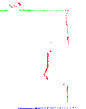The second difficulty is the correct computation of the gradient across jumping edges (see Fig. (b)). This problem is solved with a prior segmentation [16], as the gradient $\alpha_{i,j}$ is only calculated correctly if both points $\V p_{i,j}$ and $\V p_{i,j-k}$ belong to the same segment. The correct classification result can be seen in Fig. (c). Fig. shows a 3D scan with the semantic labels.

Figure: Semantically labeled 3D point cloud from a single 360$^\circ$ 3D scan. Red points mark the ceiling, yellow points objects, blue points the floor and green points correspond to artefacts from scanning the RTS/ScanDrive and the robot.