Camera Calibration

The camera is modeled by the usual pinhole approach. A camera projects a 3D point $\V p \in \RR ^3$ to the 2D image, resulting in $\V p' \in \RR ^2$. The relationship between a 3D point $\V p$ and its image projection $\V p'$ is given by

$$s \left( \begin{array}{c} \V p' \\ 1 \end{array} \right) = \M A \... ...0 & 1 \end{array} \right) \left( \begin{array}{c} \V p \\ 1 \end{array} \right) \quad \M A = \left( \begin{array}{ccc} \alpha & \gamma & u \\ 0 & \beta & v \\ 0 & 0 & 1 \end{array} \right).$$

$\M A$ is the camera matrix, i.e., internal camera parameters, with the principal point with the coordinates $(u, v)$. $\M R$ and $\V t$ specify the external camera parameters, i.e., the orthonormal $3 \times 3$ rotation matrix and translation vector of the camera in the world coordinate system. In addition to these equations, we consider the distortion, resulting in 4 additional parameters to estimate [#!zhang_2000!#].

Figure: Top: Chessboard plane for calibration. Bottom: Chessboard detection in a 3D laser range scan.

51mm

Camera calibration uses a new technique based on Zhang's method. We give a brief sketch here, details can be found in [#!zhang_2000!#]. The key idea behind Zhang's approach is to estimate the intrinsic, extrinsic and distortion camera parameters by a set of corresponding point. These 3D-to-2D point correspondences are first used to derive an analytical solution, i.e., the general $4 \times 4$ homography matrix $\M H$ is estimated:

$$s \left( \begin{array}{c} \V p' \\ 1 \end{array} \right) = \M H \left( \begin{array}{c} \V p \\ 1 \end{array} \right).$$

The estimation is done by solving an over specified system of linear equations. Since the points of 3D-to-2D point correspondences have usually small errors and only a few points are used to solve the equations for $\M H$, this first estimation needs to be optimized. A nonlinear optimization technique, i.e, the Levenberg-Marquardt algorithm based on the maximum likelihood criterion is used to optimize the error term:

$$\sum_{i=1}^n \sum_{j=1}^m \norm { \V p'_{i,j} - \V {\hat p}_{i,j}'(\M H_j)}.$$

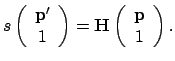
Hereby $\V p'_{i,j}$ are the points $\V p_{i,j}$ projected by $\M H_j$, and $\V {\hat p}_{i,j}$ are the given corresponding points; $i$ is the point index and $j$ is the image index. After the calculation of $\M H$, the camera matrix $\M A$, the rotation matrix $\M R$ and the translation $\V t$ are calculated from $\M H$. Again, an over specified system of linear equation is solved, followed by a nonlinear optimization of

$$\sum_{i=1}^n \sum_{j=1}^m \norm { \V p'_{i,j} - \V {\hat p}_{i,j}'(\M A, \M R_j, \M t_j)}.$$

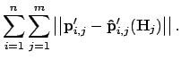
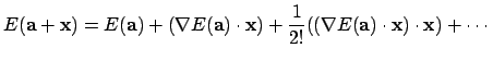
Finally the term for optimization is set to

$$\sum_{i=1}^n \sum_{j=1}^m \norm { \V p'_{i,j} - \V {\hat p}_{i,j}'(\M A, \M R_j, \M t_j, k_1, k_2, l_1, l_2)},$$

where $k_1, k_2$ are parameters for the radial distortion, and $l_1, l_2$ the ones for tangential distortion. The minimum is found by the Levenberg-Marquardt algorithm that combines gradient descent and Gauss-Newton approaches for function minimization [#!Fitzgibbon_2001!#,#!NumericalRecipes!#]. An important concept of the Levenberg-Marquardt algorithm is the vector of residuals, i.e., $\V e( \V a) = \{ E_i (\V a) \}_{i=1}{N}$, so that $E( \V a) = \norm {\V e (\V a)}$ is one of the error terms above. The goal at each iteration is to choose an update $\V x$ to the current estimate $\V a_c$, such that setting $\V a_{c+1} = \V a_c + \V x$ reduces the error $E( \V a)$. A Taylor approximation of $E (\V a + \V x)$ results in

$$E(\V a + \V x) = E(\V a) + (\nabla E(\V a) \cdot \V x) + \frac{1}{2!} ((\nabla E(\V a) \cdot \V x) \cdot \V x) + \cdots$$

Expressing this approximations in terms of $\V e$ yields [#!Fitzgibbon_2001!#]:

$$E(\V a) = \V e^T \V e$$

$$end{tex2html_deferred}$$

$$end{tex2html_deferred} \nabla E(\V a) = 2 (\nabla \V e)^T \V e$$

$$end{tex2html_deferred}$$

$$end{tex2html_deferred} \nabla^2 E(\V a) = 2 (\nabla^2 \V e) \V e + 2 (\nabla \V e)^T \nabla \V e$$

$$end{tex2html_deferred}$$

$$end{tex2html_deferred}$$

By neglecting the therm $2 (\nabla^2 \V e) \V e$ the Gauss-Newton approximation is derived, i.e.,

$$E(\V a + \V x) = \V e^T\V e + \V x^T \M J^T \V e + \V x^T \M J^T \M J \V x,$$

with $\M J$ the Jacobian matrix $\nabla e$, i.e., $J_{i,j} = \frac{\partial E_i}{\partial a_j}$. The task at each iteration is to determine a step $\V x$ that will minimize $E (\V a + \V x)$. Using the approximation of $E$ differentiating with respect to $\V x$ equating with zero, yields

$$\nabla_{\V x} E(\V x + \V a) = \M J^T \V e + \M J^T \M J \V x = 0.$$

Solving this equation for $\V x$ yields the new Gauss-Newton update $\V x = (\M J^T \M J)^{-1} \M J^T \V e$. In contrast, the update with an accelerated gradient descent is given by $\V x = \lambda^{-1} \M J^T \V e$ with $\lambda$ denoting the increment between two gradient descent steps. In every iteration this new update is calculated by a combination, i.e., by

$$\V x = (\M J^T \M J + \lambda \mathbbm{1})^{-1} \M J^T \V e.$$

For the above camera calibration algorithm the 3D-to-2D point correspondences are essential. Calibration is done with a chess board. From the image the board pattern corners are extracted automatically (Fig. 3 top). The corresponding 3D points are automatically extracted based on the corners of a quad in 3D (Fig. 3 bottom). 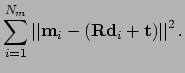The calibration algorithm extracts the 3D quad from the scanned point cloud with a modified ICP (Iterative Closest Points) algorithm [#!Besl_1992!#,#!IAV!#]. Given a set of 3D scan points $M$, a quad is matched. The algorithm computes the rotation $\M R$ and the translation $\V t$, such that the distances the scan points $\V m_{i} \in \V \RR ^3$ and their projection to the quad $\V d_i \in \V \RR ^3$ is minimized, i.e.,

$$\sum_{i=1}^{N_m}\norm {\V m_{i}-(\M R \V d_i+\V t)}^2.$$

The ICP algorithm accomplishes the minimization iteratively. It computes first the projections and then minimizes the above error term in a closed form fashion [#!Besl_1992!#,#!IAV!#]. The closed form solution is based on the representation of a rotation as a quaternion as proposed by Horn [#!Horn_1987!#].