


Next: Results and Conclusion
Up: Automatic Model Refinement for
Previous: Semantic Scene Interpretation
Due to unprecise measurements or registration errors, the 3D data
might be erroneous. These errors lead to inaccurate 3D models.
The semantic interpretation enables us to refine the model. The
planes are adjusted such that the planes explain the 3D data and
the semantic constraints like parallelism or orthogonality are
enforced.
To enforce the semantic constraints the model is first
simplified. A preprocessing step merges neighboring planes with
equal labels, e.g., two ceiling planes. This simplification
process increases the point to plane distance, which has to be
reduced in the following main optimization process. This
optimization uses an error function to enforce the parallelism or
orthogonality constraints. The error function consists of two
parts. The first part accumulates the point to plane distances
and the second part accumulates the angle differences given
through the constraints. The error function has the following
form:
 |
|
|
(4) |
 |
|
|
(5) |
 |
|
|
(6) |
 |
|
|
(7) |
|
|
|
(8) |
 |
|
|
(9) |
|
|
|
(10) |
 |
|
|
(11) |
where  expresses the parallelism (5) or
orthogonality (6) constraints according to
expresses the parallelism (5) or
orthogonality (6) constraints according to
and
 |
|
|
(15) |
Minimization of eq. (4) is a nonlinear optimization
process.
The time consumed for optimizing eq. (4) increases with
the number of plane parameters. To speed up the process, the
normal vectors  of the planes are specified by spherical
coordinates, i.e., two angles
of the planes are specified by spherical
coordinates, i.e., two angles
 . The point
  of a plane is reduced to a fixed vector pointing from the origin
of the coordinate system in the direction of and its
distance
of a plane is reduced to a fixed vector pointing from the origin
of the coordinate system in the direction of and its
distance  . The minimal description of all planes
  consists
of the concatenation of
consists
of the concatenation of  , with
 , i.e., a plane is defined by two angles and a
distance.
A suitable optimization algorithm for eq. (4) is Powell's
method (16), because the optimal solution is close
to the starting point. Powell's method finds search directions
with a small number of error function evaluations of
eq. (4). Gradient descent algorithms have difficulties,
since no derivatives are available. Cantzler et al. use a time
consuming genetic algorithm for the optimization
(6).
Powell's method computes directions for function minimization in
one direction (16). From the starting point
, i.e., a plane is defined by two angles and a
distance.
A suitable optimization algorithm for eq. (4) is Powell's
method (16), because the optimal solution is close
to the starting point. Powell's method finds search directions
with a small number of error function evaluations of
eq. (4). Gradient descent algorithms have difficulties,
since no derivatives are available. Cantzler et al. use a time
consuming genetic algorithm for the optimization
(6).
Powell's method computes directions for function minimization in
one direction (16). From the starting point  in the
  -dimensional search space (the concatenation of the
3-vector descriptions of all planes) the error function
(4) is optimized along a direction
-dimensional search space (the concatenation of the
3-vector descriptions of all planes) the error function
(4) is optimized along a direction  using a one
dimensional minimization method, e.g., Brent's method
(17).
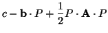
Conjugate directions are good search directions, while unit basis
directions are inefficient in error functions with valleys. At
the line minimum of a function along the direction the
gradient is perpendicular to . In addition, the
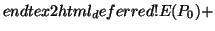
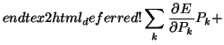
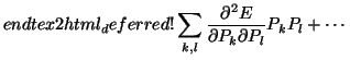
n-dimensional function is approximated at point by a Taylor
series using point as origin of the coordinate system. It
is
using a one
dimensional minimization method, e.g., Brent's method
(17).
Conjugate directions are good search directions, while unit basis
directions are inefficient in error functions with valleys. At
the line minimum of a function along the direction the
gradient is perpendicular to . In addition, the
n-dimensional function is approximated at point by a Taylor
series using point as origin of the coordinate system. It
is
 |
|
|
(16) |
|
|
|
(17) |
|
|
|
(18) |
|
|
|
(19) |
|
|
|
(20) |
|
|
|
(21) |
 |
|
|
(22) |
|
|
|
(23) |
|
|
|
(24) |
|
|
|
(25) |
|
|
|
(26) |
 |
 |
|
(27) |
|
|
|
(28) |
|
|
|
(29) |
|
|
|
(30) |
|
|
|
(31) |
 |
|
|
(32) |
 |
|
|
(33) |
 |
|
|
(34) |
 |
|
|
(35) |
![$\displaystyle end{tex2html_deferred}[1.05ex]$](img64.png) |
 |
 |
(36) |
with
 ,
,
 and
and  the
Hessian matrix of
the
Hessian matrix of  at point . Given a direction ,
the method of conjugate gradients is to select a new direction
at point . Given a direction ,
the method of conjugate gradients is to select a new direction
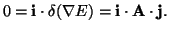
 so that and are perpendicular. This
selection prevents interference of minimization directions.
For the approximation (8) the gradient of is
so that and are perpendicular. This
selection prevents interference of minimization directions.
For the approximation (8) the gradient of is
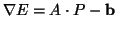 . From the differentiation (
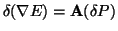 ) it follows for directions and
that
) it follows for directions and
that
 |
|
|
(37) |
With the above equation conjugate directions are defined and
Powell's method produces such directions, without computing
derivatives.
The following heuristic scheme is implemented for finding new
directions. Starting point is the description of the planes and
the initial directions  ,
,
 are the unit
basis directions. The algorithm repeats the following steps until
the error function (4) reaches a minimum
(17):
are the unit
basis directions. The algorithm repeats the following steps until
the error function (4) reaches a minimum
(17):
- Save the starting position as .
- For
, minimize the error function (4)
starting from
 along the direction and store
the minimum as the next position
along the direction and store
the minimum as the next position  . After the loop, all
are computed.
. After the loop, all
are computed.
- Let be the direction of the largest decrease. Now this
direction is replaced with the direction given by
 . The assumption of the heuristic is that the substituted
direction includes the replaced direction so that the resulting
set of directions remains linear independent.
. The assumption of the heuristic is that the substituted
direction includes the replaced direction so that the resulting
set of directions remains linear independent.
- The iteration process continues with the new starting position
 , until the minimum is reached.
Experimental evaluations for the environment test settings show
that the minimization algorithm finds a local minimum of the error
function (4) and the set of directions remains linear
independent. The computed description of the planes fits the data
and the semantic model.
The semantic description, i.e., the ceiling and walls, enable to
transform the orientation of the model along the coordinate axis.
Therefore it is not necessary to transform the model
interactively into a global coordinate system or to stay in the
coordinates given by the first 3D scan.
Next: Results and Conclusion
Up: Automatic Model Refinement for
Previous: Semantic Scene Interpretation
root
2003-08-06