The ICP algorithms spends most of its time in creating the
point pairs. ![]() D-trees (here
D-trees (here ![]() ) have been suggested to
speed up the data access [21]. The
) have been suggested to
speed up the data access [21]. The ![]() d-trees are a
binary tree data structure with terminal buckets. The data is
stored in the buckets and the keys are selected, such that a data
space is divided into two equal parts. This ensures that a data
point can be selected in
d-trees are a
binary tree data structure with terminal buckets. The data is
stored in the buckets and the keys are selected, such that a data
space is divided into two equal parts. This ensures that a data
point can be selected in ![]() . The proposed SLAM algorithm
benefits from fast data access. In addition, the time spent on
creating the tree is important.
. The proposed SLAM algorithm
benefits from fast data access. In addition, the time spent on
creating the tree is important.
For a given data set, larger bucket size results in smaller
number of terminal buckets and hence less computational time to
build the tree. The implemented algorithm uses a bucket size of
10 points and cuts recursively the scanned volume in two
equal-sized halves. Once the tree is built, the nearest neighbor
search for a given data point ![]() starts at the root of the
tree. Each tree node contains the cut dimension, i.e.,
orientation of the cut plane and the cut value. By comparing the
coordinate of the given 3D point at the cut dimension with the
cut value of this tree node, the search knows which branch to go
for next level of tree node, it will compare the cut value of
this tree node and go down further. This process is repeated
until the terminal bucket that contains the closest data points
starts at the root of the
tree. Each tree node contains the cut dimension, i.e.,
orientation of the cut plane and the cut value. By comparing the
coordinate of the given 3D point at the cut dimension with the
cut value of this tree node, the search knows which branch to go
for next level of tree node, it will compare the cut value of
this tree node and go down further. This process is repeated
until the terminal bucket that contains the closest data points
![]() is reached. It may occur, that the true neighbor lies in
a different bucket, e.g., if the distance between
is reached. It may occur, that the true neighbor lies in
a different bucket, e.g., if the distance between ![]() and a
boundary of its bucket region is less than the distance
and a
boundary of its bucket region is less than the distance ![]() and
and ![]() . In this case
. In this case ![]() d-tree algorithms have to
backtrack, until all buckets that lie within the radius
d-tree algorithms have to
backtrack, until all buckets that lie within the radius
![]() are explored. This is known as the
Ball-Within-Bounds tests [13]. The number of
distance computations is minimal for the smallest bucket size,
i.e., one point per bucket. Nevertheless the running time of a
are explored. This is known as the
Ball-Within-Bounds tests [13]. The number of
distance computations is minimal for the smallest bucket size,
i.e., one point per bucket. Nevertheless the running time of a
![]() d-tree decreases for a slightly larger bucket size. This is
due to the greater cost of backtracking as compared to a simple
linear traversal of a small list within the bucket.
d-tree decreases for a slightly larger bucket size. This is
due to the greater cost of backtracking as compared to a simple
linear traversal of a small list within the bucket.
Recently, Greenspan and Yurick introduced Approximate ![]() d-trees
(Apr-
d-trees
(Apr-![]() d-tree) [13]. The idea behind this is to
return as an approximate nearest neighbor
d-tree) [13]. The idea behind this is to
return as an approximate nearest neighbor ![]() the closest
point
the closest
point ![]() in the bucket region where
in the bucket region where ![]() lies. This value
is determined from the depth-first search, thus expensive
Ball-Within-Bounds tests and backtracking are not used
[13]. In addition to these ideas we avoid the
linear search within the bucket. During the computation of the
Apr-
lies. This value
is determined from the depth-first search, thus expensive
Ball-Within-Bounds tests and backtracking are not used
[13]. In addition to these ideas we avoid the
linear search within the bucket. During the computation of the
Apr-![]() d-tree, the mean values of the points within a bucket are
computed and stored. Then the mean value of the bucket is used as
approximate nearest neighbor, replacing the linear search.
d-tree, the mean values of the points within a bucket are
computed and stored. Then the mean value of the bucket is used as
approximate nearest neighbor, replacing the linear search.
The search using the Apr-![]() d-tree is applied until the error
function
d-tree is applied until the error
function ![]() (1) stops decreasing. To avoid
misalignments due to the approximation, the registration
algorithm is restarted using the normal
(1) stops decreasing. To avoid
misalignments due to the approximation, the registration
algorithm is restarted using the normal ![]() d-tree search. A few
iterations (usually 1-3) are needed for this final
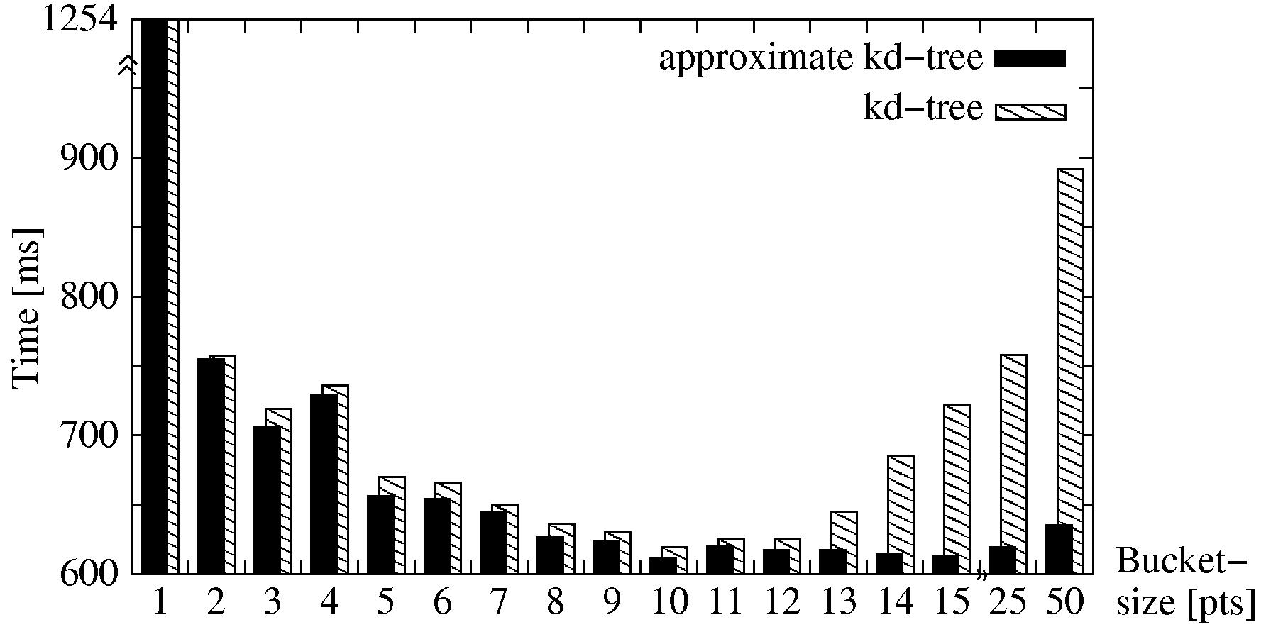
corrections. Fig. 5 shows the registration time
of two 3D scans in dependence to the bucket size using
d-tree search. A few
iterations (usually 1-3) are needed for this final
corrections. Fig. 5 shows the registration time
of two 3D scans in dependence to the bucket size using ![]() d-tree
or Apr-
d-tree
or Apr-![]() d-tree search. Both search methods have their best
performance with a bucket size of 10 points.
d-tree search. Both search methods have their best
performance with a bucket size of 10 points.
|