Powell's Method

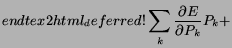
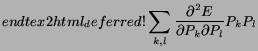
A suitable optimization algorithm for eq. (3) is Powell's method [13], because the optimal solution is close to the starting point. Powell's method finds search directions with a small number of error function evaluations of eq. (3). Gradient descent algorithms have difficulties, since no derivatives are available.

Powell's method computes directions for function minimization in one direction [13]. From the starting point $P_0$ in the $n$-dimensional search space (the concatenation of the 3-vector descriptions of all planes) the error function (3) is optimized along a direction $\V i$ using a one dimensional minimization method, e.g., Brent's method [14].

Conjugate directions are good search directions, while unit basis directions are inefficient in error functions with valleys. At the line minimum of a function along the direction $\V i$ the gradient is perpendicular to $\V i$. In addition, the n-dimensional function is approximated at point $P$ by a Taylor series using point $P_0$ as origin of the coordinate system. It is

$$$$ (14)

$$end{tex2html_deferred}!$$ (15)

$$end{tex2html_deferred}!$$ (16)

$$end{tex2html_deferred}!$$ (17)

$$end{tex2html_deferred}!$$ (18)

$$end{tex2html_deferred}!$$ (19)

$$end{tex2html_deferred}! E(P)$$ (20)

$$end{tex2html_deferred}!$$ (21)

$$end{tex2html_deferred}!$$ (22)

$$end{tex2html_deferred}!$$ (23)

$$end{tex2html_deferred}!$$ (24)

$$end{tex2html_deferred}! = $$ (25)

$$end{tex2html_deferred}!$$ (26)

$$end{tex2html_deferred}!$$ (27)

$$end{tex2html_deferred}!$$ (28)

$$end{tex2html_deferred}!$$ (29)

$$end{tex2html_deferred}! E(P_0) +$$ (30)

$$end{tex2html_deferred}! \sum_k \frac{\partial E}{\partial P_k}P_k +$$ (31)

$$end{tex2html_deferred}! \sum_{k,l} \frac{\partial^2 E}{\partial P_{k}\partial P_{l}}P_{k}P_{l}$$

$$end{tex2html_deferred}$$ (32)

$$end{tex2html_deferred} + \cdots$$

$$end{tex2html_deferred}$$ (33)

$$end{tex2html_deferred}[1.05ex] \approx c - \V b \cdot P + \frac{1}{2} P \cdot \M A \cdot P \vspace*{-1mm}$$ (34)

with $c = E(P_0)$, $\V b = \nabla E \vert _{P_0}$ and $\M A$ the Hessian matrix of $E$ at point $P_0$. Given a direction $\V i$, the method of conjugate gradients is to select a new direction $\V j$ so that $\V i$ and $\V j$ are perpendicular. This selection prevents interference of minimization directions. For the approximation above the gradient of $E$ is $\nabla E = A \cdot P - \V b$. From the differentiation ( $\delta(\nabla E) = \M A (\delta P)$) it follows for directions $\V i$ and $\V j$ that

$$\vspace*{-1mm} 0 = \V i \cdot \delta (\nabla E) = \V i \cdot \M A \cdot \V j. \vspace*{-1mm}$$ (35)

With the above equation conjugate directions are defined and Powell's method produces such directions, without computing derivatives.

The following heuristic scheme is implemented for finding new directions. Starting point is the description of the planes and the initial directions $\V i_l$, $l = 1, \ldots, n$ are the unit basis directions. The algorithm repeats the following steps until the error function (3) reaches a minimum [14]:

1. Save the starting position as $P_0$.
2. For $l = 1, \ldots, n$, minimize the error function (3) starting from $P_{l-1}$ along the direction $\V i_l$ and store the minimum as the next position $P_l$. After the loop, all $P_l$ are computed.
3. Let $\V i_l$ be the direction of the largest decrease. Now this direction $\V i_l$ is replaced with the direction given by $(P_n - P_0)$. The assumption of the heuristic is that the substituted direction includes the replaced direction so that the resulting set of directions remains linear independent.
4. The iteration process continues with the new starting position $P_0 = P_n$, until the minimum is reached.

Experimental evaluations for the environment test settings show that the minimization algorithm finds a local minimum of the error function (3) and the set of directions remains linear independent. The computed description of the planes fits the data and the semantic model.