Downhill Simplex Method

Another suitable optimization algorithm for eq. (3) is the downhill simplex method as used by Cantzler et al. [4]. A nondegenerate simplex is a geometrical figure consisting of $N+1$ vertices in $N$ dimensions, whereas the $N+1$ vertices span a $N$-dimensional vector space. Given an initial starting point $P_0$, the starting simplex is computed through

$$P_i = P_0 + \lambda \V i_l,$$ (36)

with $\V i_l$ the unit basis directions and $\lambda$ a constant that depends on the problem's characteristic length scale [14]. In our experiments $\lambda$ is set to 0.15.

The downhill simplex method consists of a series of steps, i.e., reflections and contractions [14]. In a reflection step the algorithm moves the point of the simplex where the function is largest through the opposite face of the simplex to some lower point. If the algorithm reaches a ``valley floor'', the method contracts the simplex, i.e., the volume of the simplex decreases by moving one or several points, and moves along the valley [14].

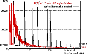
Figure 3 shows the minimization of eq. (3) with the downhill simplex method in comparison with Powell's method. The downhill simplex method performs worse during the first steps, but reaches a better minimum than Powell's method. The peaks in $E(P)$ produced by Powell's method are the result of search directions $\V i$ cross a ``valley'' in combination with large steps in Brent's line minimization algorithm.

Figure 3: Minimization of the error function starting with $E(P) = 1679.09$. Powell's method finds a minimum at 396.5 and the downhill simplex reaches a minimum at 39.0.